Calculation Methodology

01 The Question We Answer

When a commercial property sells, the county or jurisdiction may reassess it. That new assessed value drives the next property tax bill. Vental answers one underwriting question:

"If this property sold at price V, what would the jurisdiction likely tax it at next?"

Vental estimates that answer from observed comparable sales. We look at similar properties that sold, compare their sale prices to the assessed values that followed, and use that history to estimate the subject property's reassessed value and tax bill. This lets an analyst translate a purchase price into a tax expectation before the deal is underwritten.

02 How We Do It

End-to-End Flow

The total tax bill is assembled from two pieces: ad valorem tax driven by taxable value and a local rate, plus direct charges or special assessments when those parcel records are available.

Vental predicts the tax assessment ratio: the fraction of sale price that becomes taxable after reassessment. Millage rates and direct charges are looked up from public records when available. If those downstream tax facts are missing, the estimate still returns the assessment-ratio and taxable-value result.

Why We Predict a Ratio, Not a Dollar Amount

A $30M office sale and a $3M office sale produce very different tax dollars. But the ratio of post-sale taxable value to sale price is a more stable modeling target within the same county and asset class. That ratio lets the engine learn local reassessment behavior without confusing it with property size.

Building the Comparable-Sales Pool

Every estimate starts with a comparable-sales pool for the same jurisdiction and commercial asset class. Each comp is a qualified arm's length, historical sale with a next-year assessment record, so Vental can observe what happened.

Comp Influence

Not every comparable sale should have the same effect on the estimate. A comp that looks highly relevant to the subject should usually carry more influence than a comp that is technically in the pool but less representative.

What makes a comp more relevant is not universal. It depends on the jurisdiction, the asset class, and the historical sales record for that segment. In one county and asset class, prior assessment position may be the strongest signal. In another, recency, property type, or broader comp support may matter more.

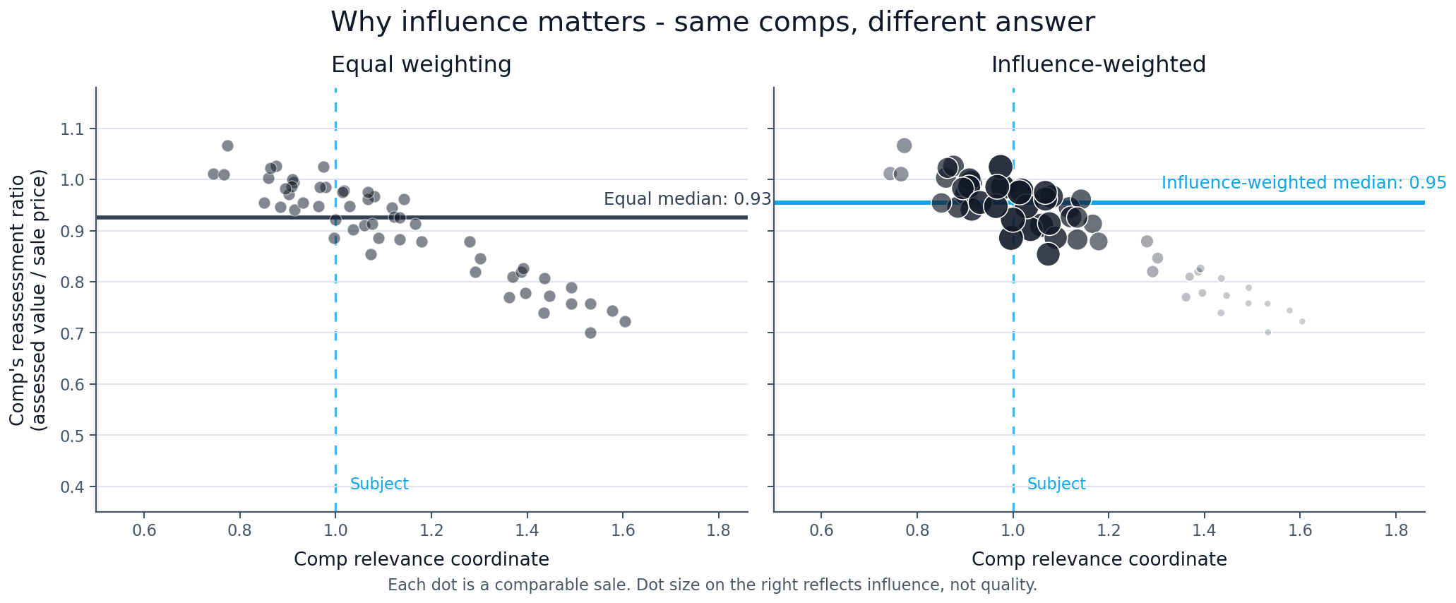
When the app shows Influence, it is not saying a comp is good or bad. It is showing how much that comp contributed to the estimate relative to the other included comps. When the app shows equal weighting, each included comp is counted the same way.

The Models

Vental's engineers and data scientists have developed several models for turning a comparable-sales pool into a prediction. Each model falls into one of three high-level classes.

• Flat mode: every included comp counts equally. There is no comp-by-comp influence score.
• Influence-weighted models: the model calculates influence from property, sale, timing, or jurisdiction-specific variables. The exact signals depend on the county and asset class.
• Factor models: comparable sales remain part of the evidence, but the final estimate is driven by calibrated property and market factors rather than a per-comp influence score.

The Vental team backtests those models by county and asset class, then the app uses the model that has worked best for that segment. A multifamily property in one county may use one model, while an office property in another county may use another.

For a detailed explanation of each model, visit the appendix.

The Prediction and Its Output

Every estimate ships with an interval around the prediction. The point estimate is Vental's best read from the comparable-sales evidence; the interval shows the reasonable range around that point estimate.

The interval is not a worst-case scenario or a guarantee. It is a practical uncertainty band based on how similar historical estimates have behaved.

A tighter interval means the comparable-sales evidence is stronger and historical outcomes have been more consistent. A wider interval means the subject is harder to match, the comp support is thinner, or similar historical outcomes have been less predictable.

Warnings and Guardrails

When applicable, Vental ships estimates with warnings that are designed to explain why the estimate is less precise or why a guarded route was selected.

Guardrails are learned offline from historical behavior. If a subject falls into a segment where one method has repeatedly underperformed, Vental can route to a lower-error fallback method and disclose that route in the result.

03 What We Don't Do

• It is not a county assessor model. Vental learns from observed post-sale outcomes, not from confidential assessor formulas.
• It does not apply owner-specific exemptions. Homestead, senior, veteran, and similar exemptions belong to owners, not the commercial property record itself.
• It does not guarantee direct charges. When non-ad-valorem or direct-charge records are unavailable, Vental clearly labels the estimate as ad-valorem only.
• It does not replace diligence. Analysts should still review the comp table, warnings, parcel facts, tax-rate source, and any planned improvements or ownership changes.

A Appendix

Select a model below for a detailed methodology note covering the model objective, key quantities, estimation procedure, output, and fallback or guardrail logic.

In these names, Pre-JV refers to the prior-year jurisdiction value ratio used as a similarity coordinate. Kernel means a smooth weighting function: comps closer to the subject on the relevant coordinates receive more influence, while distant comps fade rather than being abruptly excluded.